
Boson Examples
There are numerous public and non-public sources of geospatial and spatiotemporal data that you might wish to use: Google Earth Engine, the Esri Living Atlas, US Government Public Data (NOAA, NASA, USGS, etc). While there are several platforms to choose from that offer large scale analytics, they all have the same limitation: you need to work entirely in their platform, usually importing your own data into their platform. Combining disparate datasets from multiple sources is difficult, if not impossible. Boson makes this easy. For an overview of what Boson does, please check out this page. If you want to see some examples in action, you’re at the right place. Throughout these examples, we’ll show you how you can work with dataset from multiple different sources.
Example 1: Google Earth Engine
Google Earth Engine (GEE) is a publicly available multi-petabyte catalog of satellite imagery and geospatial datasets. Currently free for scientists and researchers, Google Earth Engine is now in general availability for commercial use as well. Google Earth Engine doesn’t just have data available, it offers analytics as well, and if you are comfortable working within their box, it’s a very capable tool which has powered some terrific research. Geodesic is a tool for bringing datasets together to answer questions - especially when those questions aren’t directly answered through use of a single data source. In the event that you want to add your own data to GEE, you have limited options. Geodesic makes it easy to include Google Earth Engine in your analysis without sacrificing the flexibility of working with other data sources as well.
The National Oceanic and Atmospheric Administration (NOAA) is responsible for monitoring weather, oceanic and atmospheric conditions, charting the seas, protecting endangered species, and many more responsibilities. Most of the data and analysis they produce is publicly available. Unfortunately, unless you have a very strong background working with climate data, they datasets can be extremely unwieldy (or impossible) to work with at scale. Even if you do have that background, some simple questions can be answered much more easily than downloading a bunch of GRIB, NetCDF, or HDF5 files from a remote FTP server, opening them up, extracting the appropriate variables, and turning them into an analysis product. Many of these datasets are curated by Google Earth Engine and stored in a format that makes them MUCH easier to work with at scale. (As an aside, we’ll also show how you can work with the raw data in the event that you need it).
Note
All examples in this page assumed you’ve imported the geodesic Python API and are working in a project. See
below
>>> import geodesic
>>> import matplotlib.pyplot as plt # Optional, for plotting
>>> _ = geodesic.set_active_project('boson-examples')
This also assumes you’re already authenticated with your identity provider
First, let’s grab the Real-Time Mesoscale Analysis dataset from GEE. RTMA is a NOAA/NWS provided dataset with a bunch of relevant variables such as temperature and wind speed/direction. If you want to access the raw RTMA data, it’s available here, but it’ll be a chore to find what we need. Fortunately, GEE packages this dataset up neatly for us.
In order to access data outside of Geodesic, we often need to create credentials. Credentials allow Geodesic to
access data that may require and account or is otherwise behind a secure API. When working with Google Earth Engine,
we operate with a bring-your-own account workflow. Every user can create as many credentials as they want and use them
when creating datasets. For details on creating credentials, see Account Management 101. For now, let’s assume
we’ve already added a GEE Service Account key using geodesic.accounts.Credential.from_gcp_service_account and
named it google-earth-engine. Adding RTMA is as simple as:
>>> rtma = geodesic.Dataset.from_google_earth_engine(
    name='rtma-gee',
    asset='NOAA/NWS/RTMA',
    credential= 'google-earth-engine',
    alias='RTMA: Real-Time Mesoscale Analysis',
    description='The Real-Time Mesoscale Analysis (RTMA) is a high-spatial and temporal resolution analysis for '
                'near-surface weather conditions. This dataset includes hourly analyses at 2.5 km for CONUS.'
)
>>> rtma.save()
Note
You can create this as above, but the Geodesic Python API will auto-populate the resulting Dataset object with
much more metadata if you have installed the GEE Python API and are logged in.
Datasets in Geodesic expose, among other things, two endpoints search and get_pixels. search searches for
features or footprints/STAC items within the dataset and get_pixels gets pixels, performing reprojection and
resampling as needed.
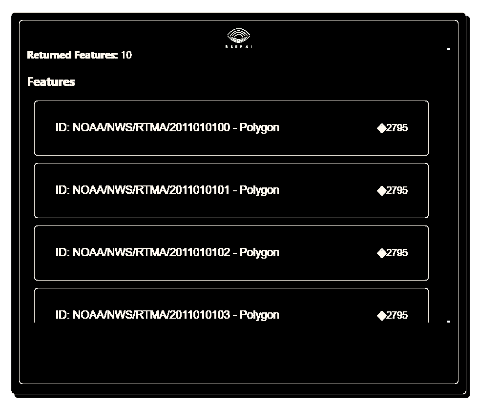
Now that the dataset is created it, we can query it just like any dataset in Geodesic. You can use a tool like bboxfinder to quickly find the bounds of region on the earth. Here we query over the state of Texas:
bbox = (-109.127197, 37.002553, -102.008057, 41.079351)
res = rtma.search(bbox=bbox)
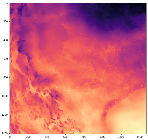
And we can get data from it as well, such as the temperature. Here we choose a pixel_size of 1000 meters. You can
set this value to whatever you wish, but all datasets have a native resolution and you aren’t buying anything by making
this number very large. It’s best to work close to the native pixel size in most situations. We let this be flexible in
order to combine disparate datasets, as we are about to show.
img = rtma.warp(
    bbox=bbox,
    datetime=('2022-12-27T00:00:00', '2022-12-27T01:00:00'),
    pixel_size=(1000, 1000),
    asset_bands=[
        {
            'asset': 'TMP',
            'bands': [0]
        }
    ]
)

# Create a quick plot of the numpy array result.
plt.figure(figsize=(10,10))
plt.imshow(img[0], cmap='magma')
Note
Some data sources, such as Google Earth Engine, have feature record count limits or image export limits. For example, Google Earth Engine is limited to 32k pixels in either dimensions and a limit of 48MB uncompressed. Boson currently adheres to these limitations as well (for GEE datasets), but we are working to resolve some of these service level differences within Boson itself. Chances are if you’re making a big request, there’s a better way to achieve the result you’re looking for,.
It’s a simple as that.
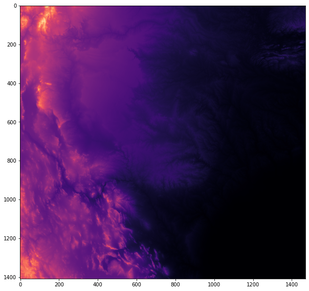
Example 2: Esri Living Atlas
Now let’s include another dataset in our “analysis”, this time turning to the Esri Living Atlas. Just for fun, let’s add a dataset of Surface Ground Elevation. As with Google Earth Engine, this dataset requires credentials to access. For ArcGIS access, the recommendation is to use OAuth2 Client Credentials, which can be created through the ArcGIS Developers portal. These can be added in a similar way as the service account for Google Earth Engine. Let’s assume we’ve done that and have a credential called agol-oauth2.
In order to get all the metadata about the ArcGIS service itself, it helps to be logged into ArcGIS Online or Enterprise using the Python API.
agol = arcgis.GIS("https://seerai.maps.arcgis.com", username="seerai")

elev = geodesic.Dataset.from_arcgis_item(
    name='surface-elevation',
    item_id='0383ba18906149e3bd2a0975a0afdb8e',
    credential='agol-oauth2',
    gis=agol
)
elev.save()

res = elev.warp(
    bbox=bbox,
    pixel_size=(1000, 1000),
    asset_bands=[
        {
            'asset': 'image',
            'bands': [0]
        }
    ]
)
Because these two datasets are created with a nearly identical command and have the exact same pixel size, it’s now trivial to ask more questions, such as: “What does the relationship between temperature and altitude at that time look like in Texas?”
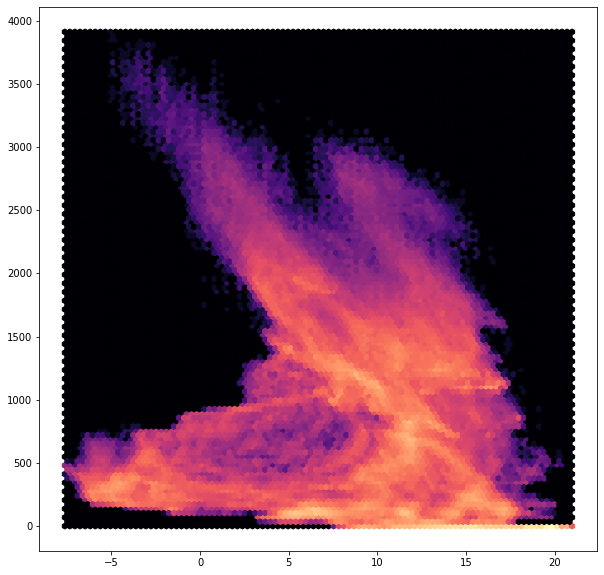
In another platform, answering this question would be time consuming and challenging. With Geodesic, it’s easy.
Boson alleviates the headaches of dealing with data from multiple sources and unifies the way you can access and work with data. Here, we created a numpy array to which we can easily apply familiar tools and methods.
Example 3: Cloud Optimized GeoTiffs
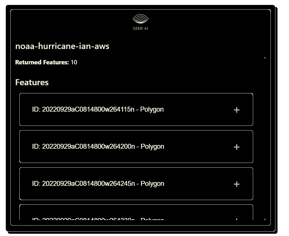
For a final example, let’s consider data that’s NOT in a standard API structure. That is, some raw data that’s not directly queryable. Boson currently enables raster files, such as Cloud Optimized GeoTiffs (COG) to be exposed for usage at scale. Let’s imagine you have your own collection of images acquired by an imaging company. If those images are placed in cloud storage, such as AWS S3, Google Cloud Storage, or Azure Blob Storage, Boson can turn them into a usable dataset. For this example, we’ll point to a public set of images, collected after Hurricane Ian by NOAA. Creating the dataset is as simple as:
ian_dataset = geodesic.Dataset.from_bucket(
    name='noaa-hurricane-ian-aws',
    url='s3://noaa-eri-pds/2022_Hurricane_Ian/'
)
ian_dataset.save()
In this case, since it’s a public S3 bucket, no credentials were required, but if the data is private, you can specify the appropriate credentials to use (IAM Account Key Pair for AWS, Service Account for GCS, Storage Account for Azure).
As long as the data is georeferenced, this is all you need to do to now use this dataset in Geodesic.
ian_dataset.search()
bbox = (-81.968551, 26.500675, -81.958337, 26.507031)
res = ds.warp(
    bbox=bbox,
    pixel_size=(0.5, 0.5),
    asset_bands=[
        {
            'asset': 'image',
            'bands': [0, 1, 2]
        }
    ]
)
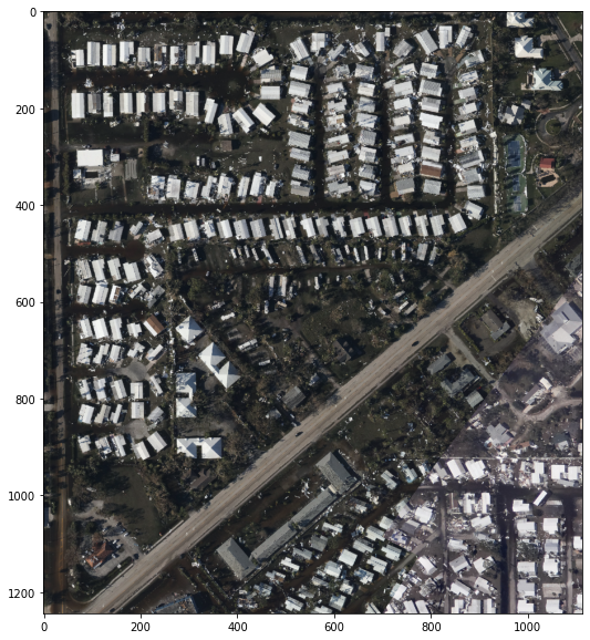
The bucket, after some brief processing time, is indexed and read for query and to export image data. Boson, as mentioned before, is built to be horizontally scalable. This means that it can run many different replicas and handle tons of requests. In this particular example, that means individual Boson distributes a large number of requests against an autoscaling cluster of Bosons. In short - Boson can keep up with very high throughput. It should be noted that while Boson itself is highly scalable, the same won’t always be true for the services referenced by Boson. You should consider this when sizing the number of workers that utilize Boson or service exceptions could happen.
There are, of course quite a few different providers for Boson and we’ve only shown a few. This list will grow, but the process of working with them is largely the same:
Provide some basic information that tells Boson where and how to access your dataset
Save to the knowledge graph
Do your analysis.
In cases where our current list of providers does not work, we provide the option to write your own. This is an entire topic in itself and we’ll cover that in a different guide. In the event you want to add your own provider to Boson, you need some place to host it, such as Google Cloud Run, AWS Lambda, or Azure Functions for serverless options, but it can be any hosting environment you wish. This allows you to maintain your own proprietary way of exposing your data, but our system doesn’t need to know the details. If this sounds like an option you need, please contact us directly.
