Working with Multiple Data Sources in your Environment of Choice - Web Map (ipyleaflet)

Boson makes bringing disparate datasets together very easy. In this demo, we will bring together data from flat files, STAC collections and ArcGIS online. Once Boson pulls the datasets together in a uniform way, we can serve them out in a variety of ways, depending on our needs.

Setup

First, let's setup the environment and create a project, if you don't already have one set up.

import geodesic
geodesic.set_active_project('tutorials')

Load the datasets

In other tutorials, we have shown how to load a variety of datasets. Here, we will make use of a few of them. In particular, we will load one dataset from a STAC collection, one from a cloud bucket, and one from an ArcGIS online service.

Load a dataset from a STAC collection

First, let's load the STAC Collection. This is Sentinel-2 L2A raster data. You can examine the tutorial in more detail in the Adding a STAC Collection tutorial, but we really only need a few lines of code:

stac_link = "https://earth-search.aws.element84.com/v0/collections/sentinel-s2-l2a-cogs"
ds = geodesic.Dataset.from_stac_collection('sentinel-2',stac_link)
ds.save()

# output:
dataset:*:*:*:sentinel-2

Load a dataset from a cloud bucket

Next, let's load a dataset from a cloud bucket. Again, you can examine the tutorial in more detail in the Adding a GeoJSON Dataset tutorial, but we can load the dataset like so:

ds = geodesic.Dataset.from_tabular_data(
    name='uscb-pop-centers',
    url='gs://geodesic-public-data/CenPop2020_Mean_CO.geojson',
    index_data=True,
    crs='EPSG:4326',
    )
ds.save()

# output:
dataset:*:*:*:uscb-pop-centers

Load a dataset from an ArcGIS online service

Finally, let's load a dataset from an ArcGIS online service. Again, you can examine the tutorial in more detail in the Adding an ArcGIS polygon_features Layer Dataset tutorial. Here is the relevant code:

url = "https://geodata.epa.gov/arcgis/rest/services/OEI/FRS_INTERESTS/MapServer/7"
ds = geodesic.Dataset.from_arcgis_layer(name = "epa-frs-locations", url=url)
ds.save()

# output:
dataset:*:*:*:epa-frs-locations

Bringing the datasets together

Even though these datasets come from different sources, Boson makes it easy to bring them together.
Now that they are saved in this project, we can serve them out in a variety of ways. We can see all the datasets we have saved in this project by using the

geodesic.boson.dataset.get_datasets method.

Let's retrieve the datasets we just saved. If you know the dataset's name, you can retrieve it by passing the dataset name to geodesic.boson.dataset.get_dataset (note the singular get_dataset). Alternatively, you can use the search parameter in

geodesic.boson.dataset.get_datasets to to query for the particular datasets we want.

from geodesic import get_datasets, get_dataset

# Return all datasets in the project
datasets = get_datasets()
datasets

# output:
DatasetList(['sentinel-2', 'uscb-pop-centers', 'epa-frs-locations', ..., 'sentinel-2-ndvi'])

# Retrieve the datasets we want
sentinel2_data = get_dataset('sentinel-2') # get_dataset with name
uscb_data = get_datasets(search='uscb-pop-centers') # get_datasets with search keyword
epa_data = get_dataset('epa-frs-locations')

Now, we can create share links to serve the data.

Serving the Datasets to a Web Map

We can serve the datasets out in a variety of ways. Let's start by simply creating feature and tile services for each dataset, and then we will serve them to an ipyleaflet map. Because Sentinel 2 data is large and contains 10 bands, we will first have to create a view of the dataset that is appropriate for serving as an feature service. "Views" allow us to apply a persistent filter to a dataset. Here, we will use the geodesic.boson.dataset.Dataset.view method to create a view that only includes the red band and a bounding box around Pennsylvania, USA for a 20-day period in January 2020.

import datetime

bbox = [-80.463867, 39.707187, -75.102539, 41.983994]
start_time = datetime.datetime(2020, 1, 1)
end_time = start_time + datetime.timedelta(days=20)

asset_bands = [{'asset': 'B04', 'bands': [0]}]

sentinel2_view = sentinel2_data.view(
    name='sentinel2-pa',
    bbox=bbox,
    datetime=[start_time, end_time],
    asset_bands=asset_bands,
)

sentinel2_view.save()

# output:
dataset:*:*:*:sentinel2-pa

Now, we can create share links to serve the data. First, we create a share token. You can set an expiration time, in seconds, for the token. Here, we will set the expiration time to 3600 seconds (1 hour). Leaving the expiration time blank will create a token that never expires.

sentinel2_token = sentinel2_view.share_as_ogc_tiles_service(3600)

Then, we can retrieve the URL for the service. Here, we will use the get_ogc_vector_tile_url method to get the URL for the vector tile service.

Geodesic also supports serving the data as a raster tile service. You can use the

:meth:get_ogc_raster_tile_url method to get the URL for the raster tile service. This requires some additional steps and will be covered in another tutorial.

sentinel2_url = sentinel2_token.get_ogc_vector_tile_url()

Next, we will create vector tile feature services for the other two datasets.

uscb_token = uscb_data.share_as_ogc_tiles_service(3600)
uscb_url = uscb_token.get_ogc_vector_tile_url()

epa_token = epa_data.share_as_ogc_tiles_service(3600)
epa_url = epa_token.get_ogc_vector_tile_url()

Finally, we can serve the datasets to an ipyleaflet map.

from geodesic import mapping
from ipyleaflet import VectorTileLayer

sentinel2_layer = VectorTileLayer(name='sentinel2-philadelphia', url=sentinel2_url)
epa_layer = VectorTileLayer(name='epa-frs-sites', url=epa_url)
uscb_layer = VectorTileLayer(name='uscb-pop-centers', url=uscb_url)

m = mapping.Map(center=[40, -75], zoom=6)
m.add_layer(sentinel2_layer)
m.add_layer(epa_layer)
m.add_layer(uscb_layer)
m

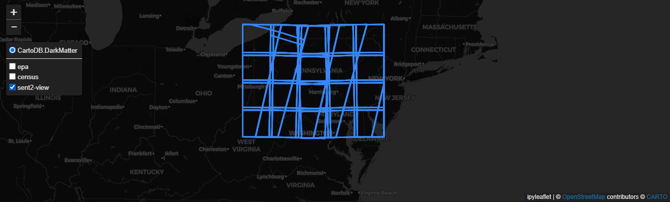
For readability, we will show the layers one at a time, starting with the Sentinel 2 imagery footprints.

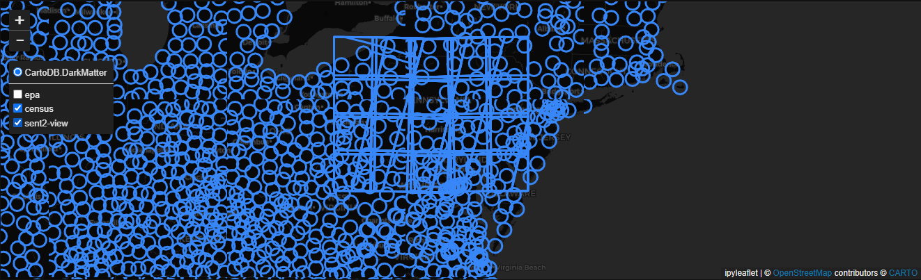
Next, we make the US Census Bureau data visible.

And finally, we add the EPA FRS layer.

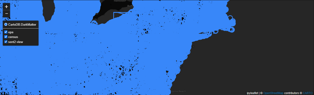
And there you have it. Using Geodesic, we've easily assembled three datasets from three different sources and served them out to the same map in a uniform way.