Running Tesseract Jobs

Tesseract is a spatiotemporal computation engine that is designed to run arbitrary processing on any data that is in the Geodesic Platform. Tesseract jobs are defined either by a JSON document or using the Geodesic Python API. In this tutorial we will go over how to make a basic Tesseract job and run it on the Geodesic Platform.

Note

This tutorial assumes that you have already installed the Geodesic Platform and have a running instance of the platform. If you have not done so, please see the Quick Start.

Creating a Tesseract Job

To create a tesseract job we use the Geodesic Python API to create and empty geodesic.tesseract.job.Job. The top level properties in the job define some of the basic information needed in the job such as the name and the output spatial reference. The job also must live in a project. When the job is run it will create a node in the knowledge graph in the particular project you specify. Lets create a tesseract-tutorial project and then a job with the name tutorial-job.

import geodesic
import geodesic.tesseract as T
from datetime import datetime
import numpy as np

project = geodesic.create_project(
    name='tesseract-tutorial',
    alias='tesseract tutorial',
    description='A project for the Tesseract jobs tutorial',
    keywords=['tesseract', 'tutorial'],
)

job = T.Job(
    name='tutorial-job',
    alias='Tutorial Job',
    description='A tutorial job to demonstrate the use of Tesseract',
    project=project,
    bbox=(-94.691162,44.414164,-94.218750,44.676466), # Southern Minnesota
    bbox_epsg=4326,
    output_epsg=3857,
)

Here we are using a bounding box that covers a portion of southern Minnesota. We are also setting the output spatial reference to 3857 which is the Web Mercator projection. This means that all outputs of the job will be transformed in to this projection. We also need to tell Tesseract which project the job should be run in. This will ensure that the output is stored in the correct project.

We need an input dataset to use in the job. This is the data that we want to prepare, then feed to a model to do some sort of processing. In this case we will use the Landsat-8 dataset. We can use the Dataset class to create a dataset in the knowledge graph that will then be available to use in any of our jobs. We will add this dataset from Google Earth Engine. You will need a Google Earth Engine credential added to Geodesic to use this data source. For more details on how to add datasets to the knowledge graph, see Boson Overview and Boson Examples.

landsat = geodesic.Dataset.from_google_earth_engine(
    name='landsat-8',
    asset='LANDSAT/LC08/C02/T1_L2',
    credential='gee-service-account',
    alias='Landsat 8 Surface Reflectance',
    domain='earth-bservation',
    category='satellite',
    type='electro-optical',
)
landsat.save()

Next we need to add a step to the job. A step is a block of work to be completed by Tesseract. Steps can be chained together to create processing pipelines and DAGs (Directed Acyclic Graphs). The first step of any job should be to create input assets. In this case we will create an input asset from the Landsat-8 dataset that we just created.

job.add_create_assets_step(
    name="add-landsat",
    asset_name="landsat",
    dataset="landsat-8",
    dataset_project=project,
    asset_bands=[
        {"asset": "SR_B4", "bands": [0]},
        {"asset": "SR_B5", "bands": [0]},
    ],
    output_time_bins=dict(
        user=T.User(
            bins=[[datetime(2021, 6, 18), datetime(2021, 6, 19)]],
        )
    ),
    output_bands=["red", "nir"],
    chip_size=1024,
    pixel_dtype=np.uint16,
    pixels_options=dict(
        pixel_size=(30.0, 30.0),
    ),
    fill_value=0.0,
    workers=1,
)

Let’s go over each of the parameters in this step.

name is what you want to call this step in the job.

asset_name is the name of the asset in the output Dataset that will be created. This means that any subsequent steps in the Tesseract job can use the asset_name to reference this asset.

dataset is the name of the dataset from the Geodesic Platform to use as input in this step. In this case this is Landsat-8. You can also provide a geodesic.entanglement.dataset.Dataset instead of the name.

dataset_project is the project that the dataset is in. In this case we are using the same project as the job. This can also be the global project for datasets that are available to all Geodesic platform users. This argument does not need to be specified if a geodesic.entanglement.dataset.Dataset object is provided for the dataset argument.

asset_bands is a list of bands to include in the asset. This parameter will depend on how the input dataset is structured. In this case we are using the SR_B4 and SR_B5 assets from the Landsat-8 dataset. The SR_B4 asset is red and the SR_B5 asset is near infrared. We also specify that we want to use the first band of each asset. This is because the Landsat-8 dataset has every band split into different assets. However, some datasets have all of their bands combined into a single asset. In that case you must specify the asset name and a list of band indices to use.

output_time_bins is used to specify how you would like the data to be binned in time. There are several different binning options available. For this job we want to use the User time binning. This allows completely user specified time bins as a list of lists. The outer list defines how many time bins there are and each inner list are the start and end of each individual bin. In this case we are using a single bin that spans from June 18st, 2021 to June 19th, 2021. This will get us a single image from the Landsat-8 dataset for the area specified in the job.

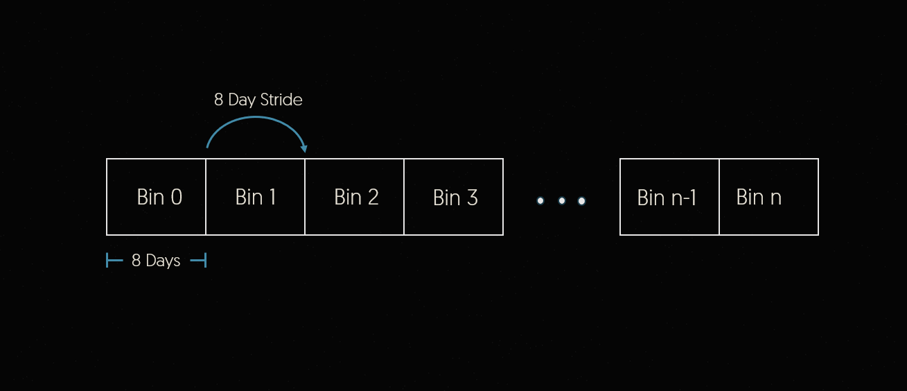
The time binning allowed in Tesseract is very flexible. You can specify any number of bins using a number of different methods. For example, the StridedBinning option which allows us to define a bin width and stide to evenly divide the time range. Here you can see that we are using 8 day bin widths with an 8 day stride. This means that each bin will contain 8 days of data and the bin start edges will be 8 days apart. This is shown in the figure below.

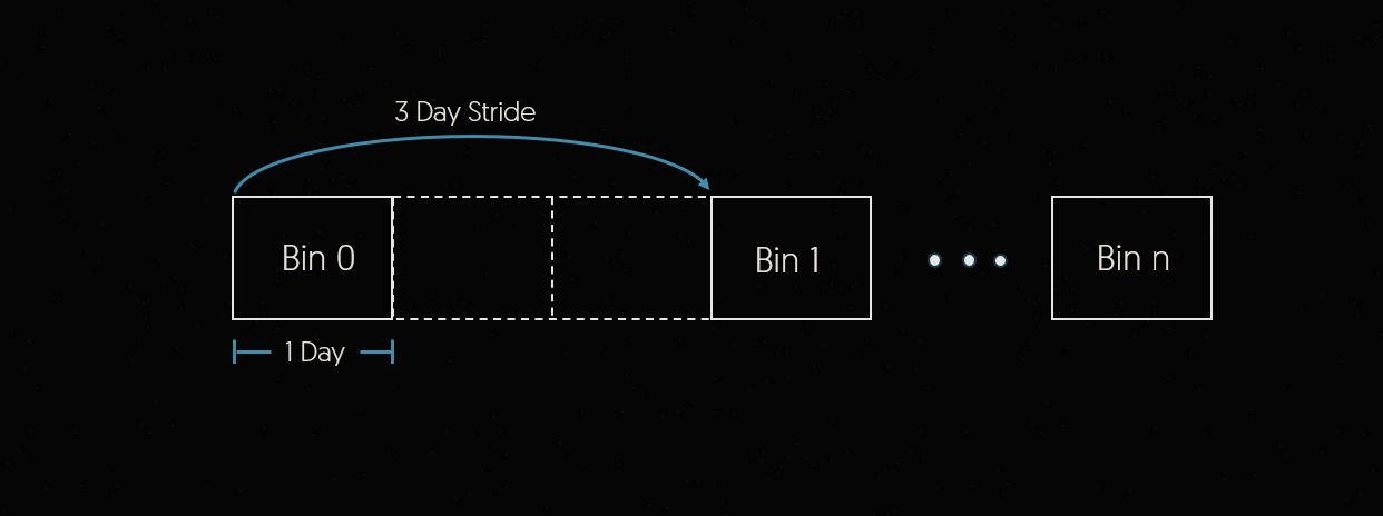
As another example, let’s imagine that for this step we wanted to have 1 day bins with a 3 day stride. This would mean that each of our bins would contain 1 day of data and the bin start edges would be 3 days apart. The result is 2 empyt bins in between the ones we requested. Any data that falls into these bins will not be included in the Tesseract job. This is shown in the figure below.

output_bands is a list of band names to use in the output asset. In this case we are using the red and nir bands. These bands will be created in the output asset.

chip_size is the size of the chips that will be created in the output data. This size is in pixels and will determine how the data is chunked. In this case we are using a chip size of 512x512 pixels.

pixel_dtype is the data type of the pixels in the output asset. This does not need to be the same as the input data type. The conversion will be done automatically in case a different dtype is required by later steps. In this case we are using uint16. Be careful not to use dtypes that could cause numerical underflow or overflow.

pixels_options is a dictionary of options that control other aspects of how the pixels are created. In this case we are setting the pixel size to 30x30 meters. The units of this parameter will always be in the units of the output spatial reference. 30 meters is the native resolution of the Landsat-8 dataset, but different values can be specified here and Tesseract will automatically resample the data. For other options available here, see geodesic.tesseract.components.PixelsOptions.

fill_value is the value to use for pixels that are outside of the input data. This should no be confused with a no_data value. Fill values are used by Zarr when reading output data from this job, but do not affect the operation of the job. In contrast, No Data values are values that are ignored during certain processing steps, such as aggregations.

workers will determine how many workers are created to complete this step of the job.

This is all that is needed to create a basic Tesseract job. This job will simpley gather the data for the requested dataset, bands, times and area which can then be retrieved as a zarr file in cloud storage. This is a great option if you are just building a dataset either for later analysis, or a training dataset to use in a deep learning model. However, we can also add more steps to the job to create a processing pipeline.

Let’s add a step to the job that will calculate the NDVI (Normalized Difference Vegetation Index) from the 2 bands that we defined on the input. NDVI is used often in vegetation health analysis and defined as:

To add a modeling step that will perform this calculation we can use the add_model_step method. This allows us to define a docker image built with the Tesseract Python SDK (details in the next tutorial) that will be used to run the model. We can also define the inputs and outputs of the model. In this case we will use the landsat asset that we created in the previous step as the input. We will also define the ndvi asset as the output. This will be the name of the asset that is created.

job.add_model_step(
    name="calculate-ndvi",
    container=T.Container(
        repository="docker.io/seerai"
        image="calculate_ndvi",
        tag="v0.0.2",
    ),
    inputs=[T.StepInput(
        asset_name="landsat",
        dataset_project=proj,
        spatial_chunk_shape=(1024, 1024),
        type="tensor",
        time_bin_selection=T.BinSelection(all=True),
    )],
    outputs=[T.StepOutput(
        asset_name="ndvi",
        chunk_shape=(1, 1, 1024, 1024),
        type="tensor",
        pixel_dtype=np.float32,
        fill_value="nan"
    )],
    workers=1,
)

Let’s go over each of the parameters in this step. We are specifically telling Tesseract that we want to create a models step which uses a container to do some sort of processing. This is different than the first step we created which just gathers, aggregates and prepares data.

name is what you want to call this step in the job.

container is a geodesic.tesseract.job.Container object that defines the docker image to use for this step. In this case we are using the seerai/tesseract-tutorial image which is available on Docker Hub. This image is built with the Tesseract Python SDK and contains a script that will calculate the NDVI from the input data. The next tutorial goes over how to build this container using the SDK.

inputs is a list of geodesic.tesseract.job.StepInput objects that define the inputs to the model. In this case we are using the landsat asset that we created in the previous step. We are also defining the time_bin_selection to be all. This means that we want to use all of the time bins in the asset. In this case since we are just calculating a band combination that doesnt depend on time, we dont actually need all of the time steps to be passed but since there are only 10, it will fit in memory easily and we can do all of them at once. We are also defining the spatial_chunk_shape to be (1024, 1024). This means that we want to process the data in chunks of 1024x1024 pixels. This shape corresponds to the chip_size parameter of the input dataset which allows for efficient processing. The model will read one chunk of input data per chunk of input to the model. There can be reasons for these two chunk sizes to be different, but in general it will be much more efficient if the chunk shapes match. This is a good size for the NDVI calculation since it is a simple calculation. However, if you are doing a more complex calculation or processing a large number of time steps, you may want to use a smaller chunk size to avoid running out of memory.

outputs is a list of geodesic.tesseract.job.StepOutput objects that define the outputs of the model. In this case we are defining the ndvi asset as the output. This will be the name of the asset that is created. We are also defining the chunk_shape to be (10, 1, 1024, 1024). This means that we want to create chunks of 10 time bins, 1 band and 1024x1024 pixels. This is the same as the input chunk shape. This means that the output chunks will be the same size as the input chunks except that we are going from 2 bands down to 1. We are also telling Tesseract that we would like the output to have the float32 data type and use nan as the fill value.

workers just like in the previous step, this will determine how many workers are created to complete this step of the job.

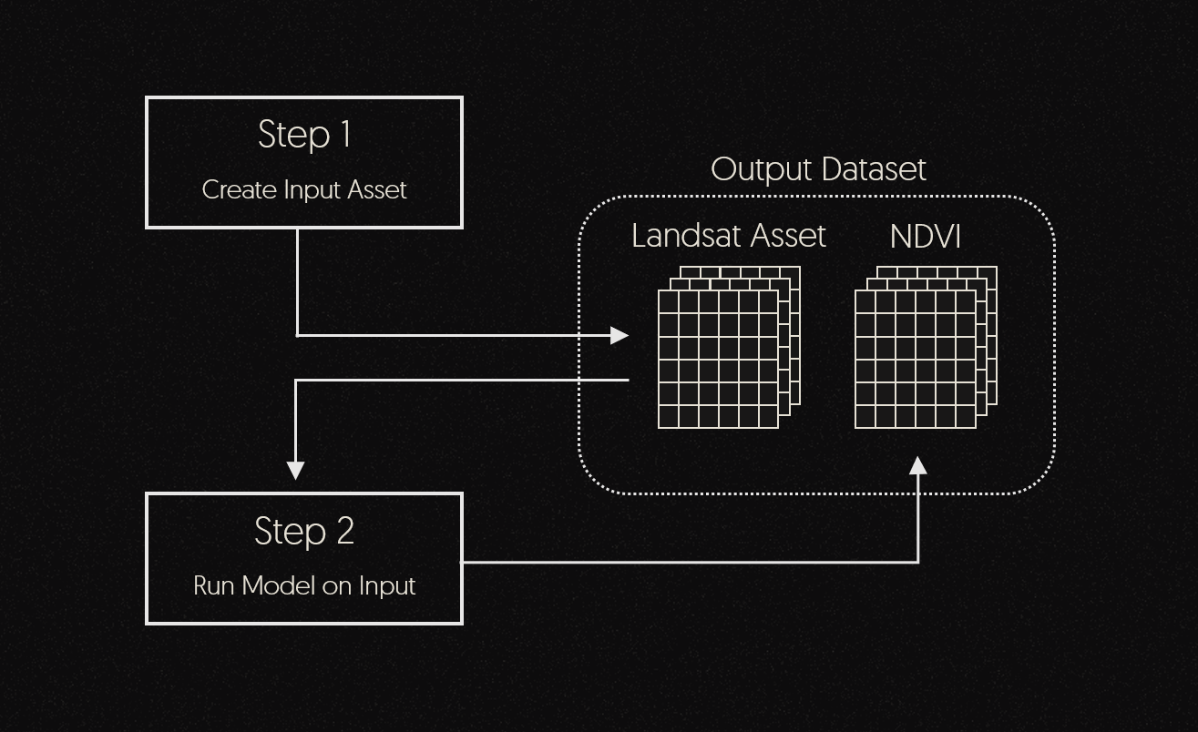
We have now defined a job that has two steps in sequence. The first step will create an asset from the Landsat-8 dataset and the second step will calculate the NDVI from the input data.

With the job defined we can now run it on the Geodesic Platform. We can use the submit method on the job.

job.submit(dry_run=True)

With the dry_run parameter set to True this will send the job description to the Tesseract service and run validation on it. This is a good way to make sure that you have defined the job correctly before submitting it. Running again with dry_run=False will submit the job and begin to spin up machines to run it. The job is first split into small units of work we call “quarks” then each quark is processed and reassembled into the output. To monitor the job as its running we can use the watch method.

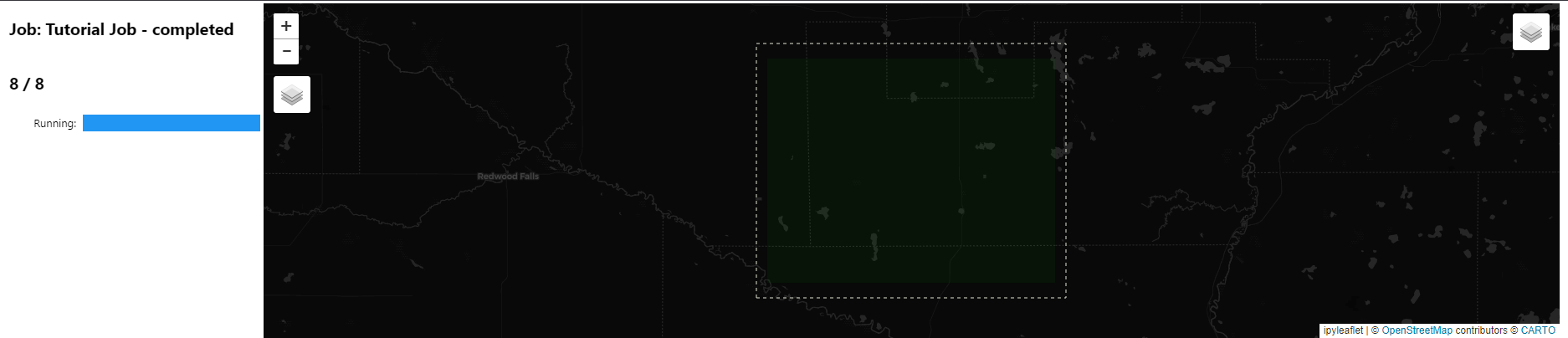
job.watch()

This will bring up a map that shows the chunks of data that will be processed. They start with a white outline and turn yellow when that chunk is being processed. When the chunk is done processing it will turn green.

You can also check the status of the job using the geodesic.tesseract.Job.status() function. This will give a simple text report with the state the job is in as well as how many quarks there are total and how many have been completed.

As soon as the job begins running, the output dataset will be available, however, until at least one quark has been processed there will be no data in the output to view. As work is completed, the dataset will be filled in. The output dataset is accessible in a few different ways. First, the output is always added to Entanglement as a new node in the knowledge graph in whatever project the job was run in. This operates exactly the same as any other dataset meaning it can be displayed on a map, queried using all available methods through Boson, or used as the input dataset in another Tesseract job.

To get the dataset that was created by the Tesseract job, you can use the function geodesic.get_objects().

objects = geodesic.get_objects()
objects

This will return a list of all of the objects in the project. You should see something like:

[dataset:earth-bservation:satellite:electro-optical:landsat-8,
dataset:*:*:*:tutorial-job]

The second object in the list is the output dataset from the Tesseract job. You can get the dataset object by grabbing the [1] index of the list. Lets take a look at what assets are in the dataset.

ndvi = objects[1]
ndvi.item['item_assets']

You should see all of the assets available in the dataset including ‘ndvi’ which is the output or our model:

{'landsat': {'description': 'Zarr formatted dataset',
     'eo:bands': [{'name': 'red'}, {'name': 'nir'}],
     'href': 'gs://tesseract-zarr/2023/12/07/eac3410e47d595abcce1269336e0174a089cee24/tensors.zarr/landsat',
     'roles': ['dataset'],
     'title': 'landsat',
     'type': 'application/zarr'},
 'logs': {'description': 'GeoParquet formatted dataset',
     'href': 'gs://tesseract-zarr/2023/12/07/eac3410e47d595abcce1269336e0174a089cee24/features/logs/logs.parquet',
     'roles': ['dataset'],
     'title': 'logs',
     'type': 'application/parquet'},
 'ndvi': {'description': 'Zarr formatted dataset',
     'href': 'gs://tesseract-zarr/2023/12/07/eac3410e47d595abcce1269336e0174a089cee24/tensors.zarr/ndvi',
     'roles': ['dataset'],
     'title': 'ndvi',
     'type': 'application/zarr'},
 'zarr-root': {'description': "The root group for this job's tensor outputs",
     'href': 'gs://tesseract-zarr/2023/12/07/eac3410e47d595abcce1269336e0174a089cee24/tensors.zarr',
     'roles': ['dataset'],
     'title': 'zarr-root',
     'type': 'application/zarr'}}

The other assets are also results of running the Tesseract Job. landsat is the input asset that was used to run the model. logs is a log of the job that was run. This can be useful for debugging jobs. zarr-root is the root of the Zarr file that contains all of the output data from the job. This zarr file will not be directly accessible unless a user specified location was used (this will be covered in an advanced Tesseract usage tutorial).

Lets use the geodesic.Dataset.get_pixels() method to read the ndvi asset from the dataset using Boson. To query this dataset we must specify at least the bounding box to be read as well as the asset that we want to read.

ndvi_pixels = ndvi.get_pixels(
    bbox=(-94.691162,44.414164,-94.218750,44.676466),
    asset_bands=[{"asset": "ndvi", "bands": [0]}],
)

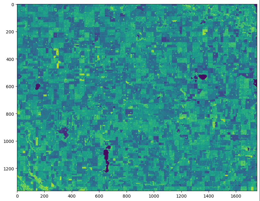
This will return a numpy array with the requested data. Let take a look at the data:

import matplotlib.pyplot as plt

fig = plt.figure(figsize=(10,10))
plt.imshow(ndvi_pixels[0])

Accessing the Zarr File Directly (Advanced)

Another way is to directly access the output files in cloud storage. Tesseract jobs that output raster data are stored as Zarr files in cloud storage. This option will only be available if you specify a location that the job should be written out to that you have credentials to access. See the output parameter of :class:`geodesic.tesseract.Job` for more information. The location of the files themselves is listed in the Entanglement dataset itself, and when using the python API the zarr() method of the job object can be used. To access a particular asset in the zarr file, you can do:

zarr_asset = job.zarr('ndvi')

This will get that asset as a Zarr group that contains a few arrays in it that contain the output data as well as metadata associated with it. Zarr arrays are accessed much like python dictionaries with the key in square brackets. The arrays you will find in the group are:

tesseract: This is the actual data array output by the model. In this example this will be the calculated NDVI value for each pixel in the input. The ‘tesseract’ asset is always a 4-dimensional array with indices (time, band, y, x). If the dataset is a non-temporal dataset then the size of dim 0 will be 1.

times: These are the timestamps (numpy.datetime64[ms]). This will be a 2-dimensional array with size equal to the number of time steps in the output dataset by 2 (n time steps, 2). The first dimension just corresponds to each time step in the output dataset and the second dimension are the bin edges for the time bin as defined in the job.

y: These are the Y (typically North-South) coordinates of each pixel in the array in the output spatial reference as defined in the job (EPSG:3857 in this example).

x: Same as above but for the X (typically East-West) coordinate.

Each of these arrays operates much the same as a numpy array. If you want to read the entire array into memory as a numpy array you can simply access all of the data using the numpy array format: np_array=zarr_asset['tesseract'][:] for example would read the entire ‘tesseract’ output into local memory. See the Zarr Documentation for more details on usage.

The assets created by Tesseract are always 4-dimensional arrays with indices (time, band, y, x). If the dataset is a non-temporal dataset, then the size of dim 0 will be 1.

Lets check the results of the job.

import matplotlib.pyplot as plt

ndvi = job.zarr('ndvi')['tesseract']
plt.imshow(ndvi[0, 0])

If at any time you restart your python kernel and lose reference to the job, you can get it again by searching all of the jobs in that project. Just use the Geodesic function geodesic.tesseract.get_jobs().

What’s Next?

In this tutorial we covered how to build a basic tesseract job and run in it on the Geodesic Platform. We created an input data asset from the Landsat-8 dataset and then ran a simple model on it giving us the output asset NDVI. In the next tutorial we will look at how to build that model using the Tesseract Python SDK.