Adding A STAC Collection Dataset

Problem

You want to use Boson to connect to a data source which is available as a STAC (SpatioTemporal Asset Catalog) Collection.

Solution

In this example, we will be accessing Sentinel 2 analysis-ready data from Earth Search by Element 84. The Sentinel 2 satellite observes the earth in 13 spectral bands once every 5 days. We will be working with the Sentinel-2 Level 2A data, which has been processed to remove atmospheric effects. The resulting data product has 10 bands and a weekly cadence. We will use Boson to access the data and produce an RGB image of a section of Philadelphia, Pennsylvania, USA.

This dataset and many others can be found on the STAC Index. Note that the geodesic.Dataset.from_stac_collection() provider requires that the STAC Collection is hosted on a STAC API endpoint, and follows the STAC specification. Specifically, the STAC URL must be of the form https://<root_url>/collections/<collection_id>.

Setup

First, we need to do some initial setup. We start by importing geodesic:

import geodesic

If you haven’t yet, you will need to authenticate geodesic using the following command:

geodesic.authenticate()

This process is covered in more detail in the Quickstart Guide.

We need to set the active project to ensure that our dataset is saved to the correct project. We do this using the uid of our desired project. If you do not know the uid, you can fetch a dictionary of existing project that you can access by running geodesic.get_projects(). Once you have the uid, you can set your active project like so:

proj = geodesic.Project(
            name="stac-collection-cookbook",
            alias="Boson from_stac_collection cookbook",
            description="Project for the from_stac_collection cookbook",
        )

proj.create()

geodesic.set_active_project(name='stac-collection-cookbook')

Creating The Provider

The Geodesic Python API provides a method, geodesic.Dataset.from_stac_collection() which makes adding a STAC collection dataset extremely straightforward. To add the Sentinel 2 Level 2A dataset, all we need is the url to the STAC Catalog. The first argument to the from_stac_collection() method is a user-specified name for the dataset, and the second argument is the url for the STAC Catalog. We simply run:

Creating The Provider

stac_url = "https://earth-search.aws.element84.com/v0/collections/sentinel-s2-l2a-cogs"

ds = geodesic.Dataset.from_stac_collection(
        name='sentinel-2',
        url=stac_url
    )

ds.save()

Testing The Provider

Now to run a quick test to ensure that the provider is working. Let’s run a simple search to check that features are returned

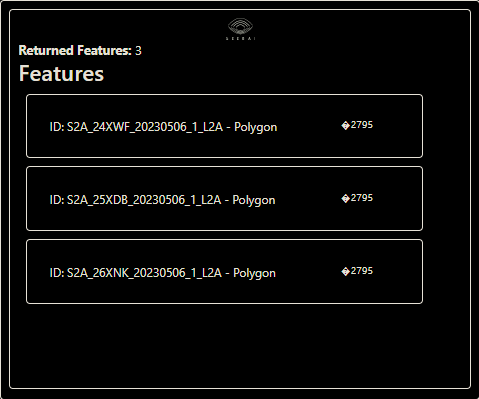
ds.search(limit=3)

This should return the first three features from the STAC collection. If you are running in a jupyter notebook, this should appear in a widget, as shown below. If you are missing the dependencies required to generate the jupyter widgets, or are not running in a notebook at all, the ds.search() method will return a dict containing the same information, which you can print to the console.

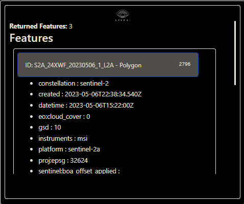
You can expand the individual features on the list to check that the correct data fields are included:

We can also inspect the Dataset with the Dataset.dataset_info() method. Let’s look at the Blue band.

Inspecting Assets

ds.dataset_info()['description']

# output:
'Sentinel-2a and Sentinel-2b imagery, processed to Level 2A (Surface Reflectance) and converted to Cloud-Optimized GeoTIFFs'

ds.dataset_info()['collections'][0]['item_assets']['B02']

# output:
{'title': 'Band 2 (blue)',
'type': 'image/tiff; application=geotiff; profile=cloud-optimized',
'roles': ['data'],
'gsd': 10,
'eo:bands': [{'name': 'B02',
'common_name': 'blue',
'center_wavelength': 0.4966,
'full_width_half_max': 0.098}]}

Creating an Image from the Dataset

We are making an RGB image, so we will pull the red, green, and blue bands from the dataset. We also need to specify the bounding box of the area we want to visualize, and set the pixel size.

Creating an Image - Setting the asset_bands

asset_bands = [
    {'asset': 'B04', 'bands': [0]}, #red
    {'asset': 'B03', 'bands': [0]}, #green
    {'asset': 'B02', 'bands': [0]}, #blue
]

The resolution is 20m per pixel in the red band, and 10m per pixel for the green and blue bands. We set the pixel size to 10m by 10m, and Boson will handle the resampling.

Creating an Image - Setting the pixel size

pixsize = [10, 10]

We will look at a section of Philadelphia, Pennsylvania, USA in September of 2020, so we will set the bounding box, start_date and end_date accordingly.

Creating an Image - Setting the bounding box and datetime

import datetime

bbox = [-75.207767, 39.934486, -75.155411, 39.970806]
start_date = datetime.datetime(2020, 9, 29)
end_date = start_date + datetime.timedelta(days=7)

We can now pull the image data using Boson.

Creating an Image - Getting the image data

boson_output = ds.get_pixels(
    bbox=bbox,
    datetime=(start_date, end_date),
    bbox_crs="EPSG:4326",
    output_crs='EPSG:3857',
    asset_bands=asset_bands,
    pixel_size=pixsize,
)

The resulting raster is a numpy array with shape of 3-bands by x-pixels by y-pixels. The first dimension represents the three color bands. We need to move them to the last dimension in order to display the image. We also need to normalize the pixel values to range between 0 and 1.

Creating an Image - Displaying the image

import numpy as np
import matplotlib.pyplot as plt

def prep_image(boson_output):
    '''
    This function accepts the numpy array from our boson request,
    and outputs a numpy array that can be displayed as an RGB image.
    Specifically, it moves the bands dimension from the first dimension
    to the last dimension, and normalizes the data to be between 0 and 1.
    '''

    rgb_data = np.transpose(boson_output, (1, 2, 0))
    rgb_data = (rgb_data - np.min(rgb_data)) / (np.max(rgb_data) - np.min(rgb_data))

    return rgb_data

rgb_image = prep_image(boson_output)
plt.imshow(rgb_image)
plt.show()

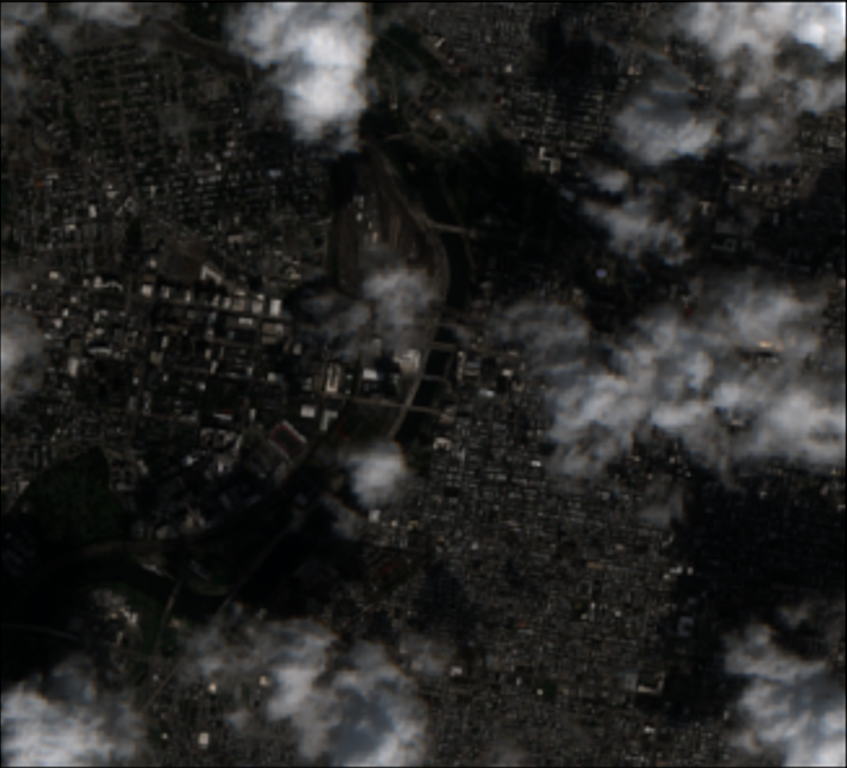
This image has some scattered clouds. Let’s grab some more images and make a composite to remove the clouds. We will grab images for 3 weeks, starting on 9/5/2020.

Creating an Image - Making a composite image

start_date_list = [datetime.datetime(2020, 9, 5) + datetime.timedelta(days=7 * time_step) for time_step in range(3)]

rgb_images = []

for start_date in start_date_list:

    end_date = start_date + datetime.timedelta(days=7)

    boson_output = ds.get_pixels(bbox=bbox,
                    datetime=[start_date, end_date],
                    content_type='raw',
                    bbox_crs='EPSG:4326',
                    output_crs='EPSG:3857',
                    asset_bands=asset_bands,
                    pixel_size=pixsize)

    rgb_image = prep_image(boson_output)
    rgb_images.append(rgb_image)

    start_date = end_date


composite_image = np.median(rgb_images, axis=0)
plt.imshow(composite_image)
plt.show()

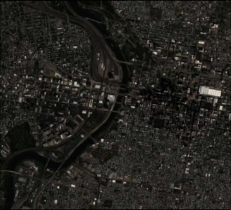
In this cloudless image, you can see the Schuylkill River dividing West Philadelphia from Center City. The large white rectangle to the east is the Pennsylvania Convention Center.