Accessing raster data with Dataset.get_pixels¶

Problem¶

You want to access raster data from a Boson Dataset.

Solution¶

In this example, we will be accessing Sentinel 2 analysis-ready data from Earth Search by Element 84. The Sentinel 2 satellites together observe the earth in 13 spectral bands, with each satellite capturing imagery once every 5 days. We will be working with the Sentinel-2 Level 2A data, which has been processed to remove atmospheric effects. The resulting data product has imagery for every 2-4 days in 10 spectral bands. We will use Boson to access the data and examine the NDVI (Normalized Difference Vegetation Index) over some corn fields in Idaho. NDVI is a measure of crop health in an area, and is calculated from the red and near-infrared bands of the satellite data.

Setup¶

The process of accessing Sentinel 2 data and saving it as a Boson Dataset is covered in the Adding a STAC Collection Dataset cookbook. Please follow that cookbook up through the “Testing the Provider” section to create the dataset.

Creating an Image from the Dataset¶

We are making an NDVI image, so we will pull the red and near-infrared (NIR) bands from the dataset. We also need to specify the bounding box of the area we want to visualize, and set the pixel size.

Creating an Image - Setting the asset_bands¶

asset_bands = [
    {'asset': 'B04', 'bands': [0]}, #red
    {'asset': 'B08', 'bands': [0]}, #nir
]

The resolution is 20m per pixel in the red band, and 10m per pixel in the NIR. We set the pixel size to 10m by 10m, and Boson will handle the resampling.

Creating an Image - Setting the pixel size¶

pixsize = [10, 10]

We will look at some corn fields in Idaho, USA in September of 2020, so we set the bounding box, start_date and end_date accordingly.

Creating an Image - Setting the bounding box and datetime¶

import datetime

bbox = [-116.730895,43.550601,-116.718450,43.561362]

start_date = datetime.datetime(2020, 9, 1)
end_date = start_date + datetime.timedelta(days=7)

We can now pull the image data using Boson.

Creating an Image - Getting the image data¶

boson_output = ds.get_pixels(
    bbox=bbox,
    datetime=(start_date, end_date),
    bbox_crs="EPSG:4326",
    output_crs="EPSG:3857",
    asset_bands=asset_bands,
    pixel_size=pixsize,
)

The result is a numpy array that is 2-bands x 165-pixels x 139-pixels. We need to calculate the NDVI, and display the image.

Creating an NDVI Image - Displaying the image¶

import matplotlib.pyplot as plt

def create_ndvi_image(boson_output):
    '''
    Accepts Boson output and returns an NDVI image.
    We add 1e-9 to the denominator of the NDVI calculation
    to avoid division by zero.
    '''

    red = boson_output[0, :, :]
    nir = boson_output[1, :, :]

    ndvi = (nir - red) / (nir + red + 1e-9)

    return ndvi

first_ndvi_image = create_ndvi_image(boson_output)
plt.imshow(first_ndvi_image)
plt.title('NDVI of Corn Field in Idaho')
plt.colorbar()
plt.show()

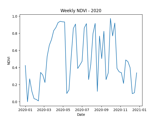
Analyzing NDVI with Boson¶

We can examine the NDVI over time by pulling weekly images and calculating the median NDVI for each image.

NDVI Time Series¶

import numpy as np

start_date_list = [datetime.datetime(2020, 1, 1) + datetime.timedelta(days=time_step * 7) for time_step in range(52)]

ndvi_images = []

for start_date in start_date_list:

    end_date = start_date + datetime.timedelta(days=7)

    boson_output = ds.get_pixels(bbox=bbox,
                    datetime=[start_date, end_date],
                    bbox_crs="EPSG:4326",
                    output_crs="EPSG:3857",
                    asset_bands=asset_bands,
                    pixel_size=pixsize)

    ndvi_image = create_ndvi_image(boson_output)
    ndvi_images.append(ndvi_image)

    start_date = end_date

ndvi_median_series = [np.median(ndvi_image) for ndvi_image in ndvi_images]

# Plot the NDVI time series
plt.plot(start_date_list, ndvi_median_series)
plt.xlabel('Date')
plt.ylabel('NDVI')
plt.title('Weekly NDVI - 2020')

plt.show()

Get Pixel Options¶

Now that we have accessed and analyzed the data, let’s look more closely at some of the options we can use with the Dataset.get_pixels() method.

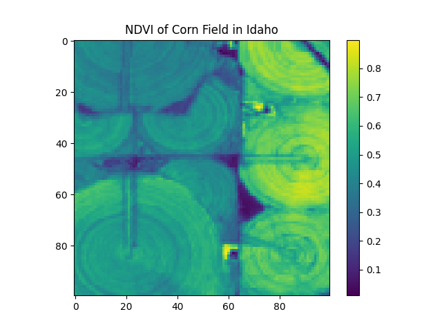
pixel_size vs. shape¶

Above, we set the pixel size to 10m by 10m. This means that each pixel in the resulting image represents a 10m by 10m area on the ground. Suppose, however, that we need the array to be a particular shape. We can set the shape parameter to specify the number of pixels in the x and y directions, and Boson will automatically resample the data to fit the new shape. Only one of pixel_size or shape can be set.

output_shape = [100, 100]

start_date = datetime.datetime(2020, 9, 1)
end_date = start_date + datetime.timedelta(days=7)

boson_output = ds.get_pixels(
    bbox=bbox,
    datetime=(start_date, end_date),
    bbox_crs="EPSG:4326",
    output_crs="EPSG:3857",
    asset_bands=asset_bands,
    shape=output_shape
)
ndvi_image = create_ndvi_image(boson_output)

plt.imshow(ndvi_image)
plt.title('NDVI of Corn Field in Idaho')
plt.colorbar()

plt.show()

output_crs¶

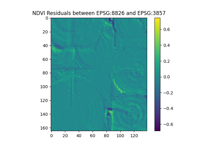
Thus far, for the output coordinate reference system (CRS), we have been using EPSG:3857, which is the Web Mercator projection, also called WGS 84. This is the default, and is the most common projection for web maps. But suppose we want to use a more accurate CRS for Idaho, such as the Idaho Transverse Mercator projection, EPSG:8826. We can set the output_crs parameter to this value. Boson will automatically reproject the data to the new CRS. In order to compare the new output to the original NDVI image, we will need to set the shape parameter to match the original image shape, as the number of pixels in the x and y directions will change.

Using a different output_crs¶

start_date = datetime.datetime(2020, 9, 1)
end_date = start_date + datetime.timedelta(days=7)

boson_output_8826 = ds.get_pixels(
    bbox=bbox,
    datetime=(start_date, end_date),
    bbox_crs="EPSG:4326",
    output_crs="EPSG:8826",
    asset_bands=asset_bands,
    shape=first_ndvi_image.shape
)

ndvi_image_8826 = create_ndvi_image(boson_output_8826)
difference_image = ndvi_image_8826 - first_ndvi_image

plt.imshow(difference_image)
plt.title('NDVI Residuals between EPSG:8826 and EPSG:3857')
plt.colorbar()
plt.show()

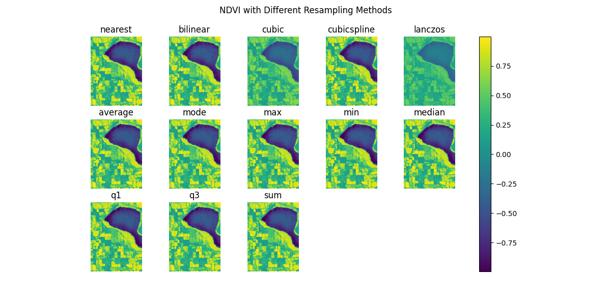
../../_images/ndvi_residuals_output_crs.png

resampling¶

By default, Boson will capture all images that intersect the bounding box and datetime range, and resample them to the output pixel size. Its default behavior is to use the nearest neighbor resampling method. We can change this behavior by setting the resampling parameter to a different value. The resampling methods are based on those found in GDAL, and include nearest, bilinear, cubic, cubicspline, lanczos, average, mode, max, min, median, q1, q3, and sum. For this example, we will zoom out a bit to see the effect of the different resampling methods.

Using a different resampling method¶

start_date = datetime.datetime(2020, 9, 1)
end_date = start_date + datetime.timedelta(days=14)
bbox = [-116.765895, 43.515601, -116.68345, 43.596362]

fig, ax = plt.subplots(3, 5, figsize=(12, 6))

resampling_methods = ['nearest', 'bilinear', 'cubic', 'cubicspline', 'lanczos', 'average', 'mode', 'max', 'min', 'median', 'q1', 'q3', 'sum']

for i, method in enumerate(resampling_methods):
    boson_output = ds.get_pixels(
        bbox=bbox,
        datetime=(start_date, end_date),
        bbox_crs="EPSG:4326",
        output_crs="EPSG:3857",
        asset_bands=asset_bands,
        pixel_size=pixsize,
        resampling=method
        )
    ndvi_image = create_ndvi_image(boson_output)
    ax[i//5, i%5].imshow(ndvi_image)
    ax[i//5, i%5].set_title(method)
    ax[i//5, i%5].axis('off')

ax[2, 3].axis('off')
ax[2, 4].axis('off')
fig.suptitle('NDVI with Different Resampling Methods')
plt.show()